Online Self-Tuning PID Controller
|
|
|
|
|
|
|
Introduction

(View more Control information or download preliminary software modules.)
A previously posted note on this site describes an experimental PI controller augmented with automatic self-tuning features [1]. Why not a PID controller? This article explains why. It also shows how a classic tuning strategy, unsatisfactory in itself, makes a useful complement to the self-tuning strategy, extending the method to full PID control.
Why Not Just Extend the Original Method?
We did that. We were not happy with the results.
In theory, the iterative feedback technique [2] used for the self-tuning PI controller [1] is equally valid for PID controllers or any kind of
low order controller. Whatever the tuning parameters are, you
have to expand the math and derive the filters to estimate
the required gradient terms, but this is basically an
algebraic exercise. Adding an additional new gradient term for
the Td gain should nicely extend the
PI method to cover PID.
Problem of Estimation and Noise
The transfer function for a derivative operator in the
Laplace frequency domain is s, with a zero at the
origin point. Applied to sinusoidal waveforms, the magnitude of
response to a frequency w is |w|
— in other words, the higher the frequency, the greater
the response. Very small levels of wideband noise (even the
quantization chatter from digitizing analog signals) can be
blown grossly out of proportion.
In the iterative feedback scheme, the filters for estimating
the gradient of the D-term gain have an s2
term, the equivalent to two derivative operations in
series. The problems of estimating this second derivative are
much worse. The response to noise is terrible. There are some
things you can do to improve the estimates, but they involve
calculations that are difficult for online applications in real
time.
Problem of Cross-Purposes
If you are familiar with the effects of PID gains (see for example the tutorial article [3] on this site), you know that when a system is operating too close to its stability limit, it tends to oscillate. Some reasonable tuning strategies to correct this are
- reduce the integral gain to reduce phase shifts.
- increase the derivative gain to improve damping.
Similarly, if the system response is too heavily damped and sluggish, try the opposite.
- increase the integral gain to respond more quickly.
- decrease the derivative gain to reduce excess damping.
The integral feedback and derivative feedback adjustments tend to adjust in the same manner except opposite in sign. Maybe one should be adjusted more than the other, but the gradient will have difficulty discovering this. It tends to follow the patterns above, ratcheting the integral gain up and the derivative gain down, then ratcheting the integral gains down and the derivative gains up, responding to slight variations in the data. Maybe none of the results are particularly bad, but there is little progress toward stable gain settings. The wandering is easily driven by the noise from the estimator filters.
Raising The Dead
Can we substitute a more productive behavior than the "wandering" driven up and down by noise? Strangely enough, we can draw motivation from a very old source: PID tuning rules.
Another technology article on this site treats the historical Z-N Tuning Rule [4] rather rudely. The underlying idea isn't bad, it is just that the assumptions under which the rule is valid usually lie so far from reality that it is hard to take the results seriously. However, we can observe that, in the end, the tuning rules select integral and derivative time constant parameters using formulas of the form
    Ti  =  C1 * Tc
    Td  =  C2 * Tc
where Tc is the period of the
critical frequency at the stability margin, and constants
C1 and C2 are "magic values"
established by the tuning rule. Combining these relationships
tells us that the integral and derivative gains are selected in
fixed proportions.
Td = C2/C1 * Ti
The value of the C2/C1 ratio affects the nature
of the tuning but is apparently not critical. Various heuristic
tuning rules in the Z-N rule family recommend different values,
though the range does not vary by much.
| Rule | Gain Ratio |
|---|---|
| Classic Ziegler-Nichols Rule | 0.25 |
| Pessen Integral Rule | 0.38 |
| Some Overshoot Rule | 0.67 |
A heuristic observation based on the tuning rules:
Provided that the fundamental nature of your system does not change drastically over time, the ratio of integral to derivative gains will be about the same in any good PID loop tuning for your system.
What is the best ratio? You will have to make that determination, depending on your system. It seems reasonable to start with something roughly in the middle of the range that works for Ziegler-Nichols-style tuning rules — 0.4 for example. If you are not satisfied with the results, try values of 0.2 and 0.6 and compare.
Integration Into the Self-Tuning Controller
To include the tuning ratio heuristic in the self-tuning PI
controller, start with the PIZST command
and modify its damping gain term. In the original command, the
damping gain was a fixed gain value Td
. In the new command form called PIDZST,
this parameter is replaced by ratio, the
scaling factor applied to the Ti
gain term to derive the Td gain
value. The gradient computations are as
described for P-I tuning [1] . However, after applying
incremental gain adjustments to the other gain
terms, the derivative gain is adjusted to conform to the gain
ratio heuristic.
Without formal proof of convergence for this approach, testing has shown that it converges very much like the original P-I controller tuning. There appears to be no particular reason to use both command forms. If you don't want to use the derivative gain term, just set the gain ratio parameter value to zero.
Test Case
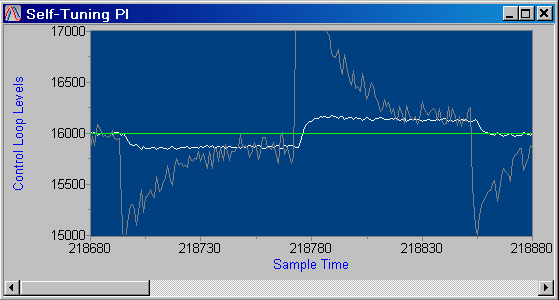
For a baseline case, the gain ratio parameter is set to 0 in a simulation of a sluggish, noisy low order system under closed loop control. This disables the derivative term, yielding the same tuning result as the original P-I configuration. The self-tuning process is allowed to run to convergence. At this point, its response to small online step disturbances is shown in Figure 1.
Figure 1 - Self-tuned PI Control
Now the tuning ratio parameter is set to the value 0.35, enabling the derivative control action according to the tuning heuristic. The experiment is repeated. After tuning, the step disturbance responses are as shown in Figure 2
Figure 2 - Self-tuned PID Control

You can see that there are some subtle differences.
- The extra damping allows a slightly higher integral gain, so the initial transient is a little faster.
- The final settling is just slightly faster. In the PI response, you can see some curvature about halfway through the pulse disturbance. In the PID response, the curvature is visible about 1/3 of the way.
- The tuned PID response has an initial overshoot, typical of tuning rules. You can use a different gain ratio to get more overshoot or less.
That the results are not dramatically different is no surprise. The differences are basically between using or not using derivative gain in PID loops. Sometimes the benefits are significant, sometimes not.
Conclusions
The self-tuning PID controls can be well suited for systems in which
- PI or PID controls are suitable.
- PID controls are slightly better than PI controls when well tuned.
- the essential character of the system response remains about the same over time.
- system parameters change slowly over time so loop tuning adjustments are needed.
The implementation is an interesting example of the flexibility of a DAPL processing command for implementing a control strategy. A theoretically appealing feature doesn't want to work out? With the implementation available in the form of a maintainable DAPL processing command, you can fix the problem. You don't have to throw away everything and start over.
Adaptive and self-tuning methods seem inherently risky. They
change — into what? Can you trust them to change in a
beneficial way? To give the PIDZST command a
through workout and let it prove what it can do, you can
download a copy to run on your Data Acquisition Processor
system. If you don't have a Data Acquisition Processor system,
consider calling us to make arrangements
for a test system.
Footnotes and References:
- Online Self-Tuning PI Controller, an article on this site, discussing an online, self-testing and self-tuning controller that uses a variation of the iterative feedback method in combination with a fully-automated injection tests.
- "Iterative Feedback Tuning: Theory and Applications" (linked to Abstract) in Control Systems Magazine, IEEE, Volume 18, Issue 4, August 1998, pp. 26-41.
- Tuning PID Control by Simulation. While this technical note has little to offer (yet) for practical loop tuning, it does show useful before-and-after illustrations of the effects of each gain term.
- Ziegler-Nichols Tuning Rules for PID, on this site. Explains the basics and dangers of this easily implemented but undependable tuning approach.
Return to the Control page.