Calibrating Thermistor Sensors
|
|
|
|
|
|
|
Calibrate Thermistors


Thermistors have the advantage of a very high sensitivity to temperature changes, but the disadvantage of an aggressively nonlinear characteristic. Here is a characteristic curve showing the resistance of a typical negative temperature coefficient thermistor device over a temperature range from 0 to 100 degrees C.
Figure 1 - Typical thermistor curve
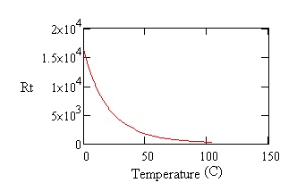
As you can see, the value changes from over 15k ohms to under 100 ohms. The change is most rapid at low temperatures, giving great resolution for determining the corresponding temperature values there. At the other end of the range, resistance levels change relatively less with temperature and measurement resolution is relatively poor.
Curve forms are available that describe the nonlinear shape of
the thermistor characteristic quite well. The most commonly used form is the
Steinhart-Hart Equation. The resistance measurement of the
thermistor is not normalized, so just use the measured value of
Rt in ohms. Manufacturers can provide typical values of
the ka, kb, and kc coefficients, or you
can calibrate these values for better accuracy.
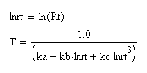
Steinhart-Hart Equation
Thermistor Linearization Curves
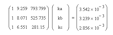
It is relatively easy to calibrate your own response curves, if you have an accurate temperature measurement standard. Convert the temperature values to Kelvins, and invert. Take the corresponding measured resistance values and compute the natural logarithm. Now, fit the coefficients of a third order polynomial in the log-resistance values to best match the inverse-temperature values.
For the following example, three points are selected, two close to the ends of the operating range and one near the center. We know that measurements will not be completely accurate, so artificial errors have been inserted into the data to result in temperature errors of magnitude 0.1 degrees C with alternating sign at the three measured points.
Data with artificial 0.1 degree errors added
| Resistance | Temperature |
|---|---|
| 10500 | 9.13 |
| 3200 | 35.56 |
| 700 | 77.02 |
Powers of log-resistance are collected in a matrix,
and the inverses of temperature in Kelvins are collected in a
vector. The model coefficients ka, kb, and
kc are obtained by solving the following matrix
equation.
| Term | 3-point Fit |
Actual Curve |
|---|---|---|
| ka | 1.236*10-3 |
1.283*10-3 |
| kb | 2.453*10-4 |
2.362*10-4 |
| kc | 4.389*10-8 |
9.285*10-8 |
Both of these formulas produce curves that are virtually indistinguishable from Figure 1. The following shows the differences — the calibration errors — that resulted from the data errors deliberately included for the the 3-point fit.
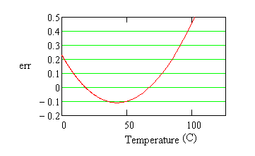
Figure 2 - Fitting error in degrees
Deviations of 0.1 degrees appear, as we know they should, where they were injected at the locations of the measured points used for the fit. At intermediate locations, the fit error is well behaved. We can conclude that the fit is about as good as the measurement errors that went into making it — but don't extrapolate much beyond the range that you measure. To reduce sensitivity to noise during calibration try the following steps.
- Calibrate over a range just a little wider than the range you intend to use.
- Select some points very close to the limits of the range you intend to use.
- Take multiple measurements at each point and average to reduce random noise.
- Consider using more than three points, and determining best-fit coefficients using least-squares methods.
Balancing measurement resolution
The linearization takes care of the problem of interpreting the highly nonlinear response, but not the problem of uneven measurement resolution.
If the range is not too large, you can balance the resolution significantly by measuring in a voltage divider configuration. Power the thermistor from a regulated voltage supply, connect the other end to ground through an accurately measured load resistance, and observe the output voltage where the thermistor and load resistor join.
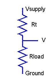
Figure 3 - Voltage divider network
The goal is to obtain a relatively uniform relationship between temperature and measured voltage. The linearization curves will take care of the rest. The following shows the relationship between temperature and measured voltage with a load resistor that is about half of the nominal room-temperature resistance.
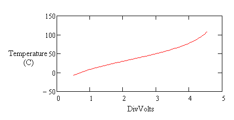
Figure 4 - Flattened thermistor response in divider network
The slope doesn't change much through the operating range. This is very different from the drastic nonlinear behavior you see in Figure 1. How does this work? The voltage divider has a saturating characteristic that responds less as thermistor resistance grows. The growth and saturation effects approximately balance.
Measure a temperature using a thermistor device in the voltage divider configuration by doing the following.
- Calculate the current flow from the measured voltage and accurately known load resistance.
- Determine the thermistor resistance from the voltage across it and the known current.
- Apply the Steinhart-Hart equation, either with nominal values provided by the manufacturer, or with adjusted values determined from calibration, to obtain the temperature reading.
- Optionally: convert temperature units from Kelvins to degrees C or degrees F.
You can use the DIVIDER command, available on this site, for computing the resistance value given the measured voltage
level in a voltage divider configuration. You can use the THERMISTOR command, also available on this site, for computing the Steinhart-Hart curves using typical or calibrated
coefficients.