Thermocouple Application
|
|
|
|
|
|
|
Fast, Accurate Thermocouple Measurement


This application example is based on a commercial HTST (High Temperature, Short Time) pasteurization processing for milk. We will cover only the temperature measurement aspects. The basic HTST process must do the following:
- Heat the milk quickly from a holding temperature to the required temperature for destroying microbes and harmful enzymes (for example 72 degrees C).
- Holding the milk at this temperature, pass it through a length of tubing at a closely controlled flow rate.
- The milk exits the process at the far end of the tubing, after the required time interval (for example 22 seconds).
- If the milk is still at the required temperature at the exit point, it is allowed to continue on for further processing.
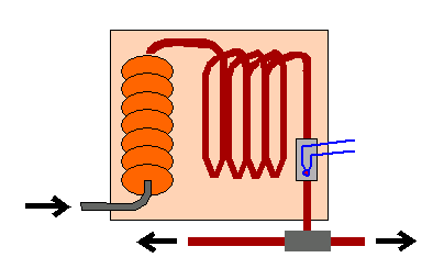
Figure 1 - HTST pasteurization process
The processing is temperature critical. If the temperature is too low, there are public safety and product quality concerns. If the temperature is too high, energy is wasted and the product can be damaged. If instruments respond too slowly, some inadequately treated milk could pass the exit valve before a problem is detected.
The basic application requirements for the temperature measurement are:
- Operating range of 55 degrees to 85 degrees C.
- No physical damage from out-of-range temperatures.
- Total measurement accuracy +- 0.5 degrees C.
- Long term drift +- 0.2 degrees C.
- Maximum settling time 4 seconds.
Selecting a sensor
A high quality type T thermocouple probe is selected. Thermistors have good response characteristics but are vulnerable to moisture and damage. RTDs have better stability and linearity, but slow response times — perhaps this is because the entire RTD has to settle to thermal equilibrium before a reading is accurate, whereas only a thermocouple probe tip needs to settle to temperature.
High quality type T thermocouple probes can be calibrated to an accuracy of about 0.1 degrees C. These use very fine gage wires that can reach a thermal equilibrium quickly. To prevent chemical interaction with the milk products there must be a protective cover. This will degrade the thermal response rate significantly, but if the resulting time constant remains under 0.5 seconds, the settling time requirement is met easily.
The main challenge with a thermocouple sensor is the very low signal level, difficult to isolate from background noise.
Thermocouple cold junctions
Thermocouples have a fundamental limitation that they measure a temperature difference rather than an absolute temperature. To know the temperature of the milk, it is necessary to know the reference temperature at the thermocouple cold junction. The usual approach of measuring the cold junction with a solid-state device located on a termination board near the cold junction terminals is not satisfactory for this application, because the solid-state sensors have a baseline error of +- 0.5 degrees C, allowing no room for device calibration errors, measurement noise, or any other error source.
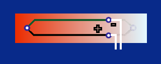
Figure 2 - Thermocouple measurement without reference junction
The issue of how to obtain an accurate cold junction measurement is covered in a separate note. We will merely presume here that there is a separate temperature measurement involved, and that the cold junction absolute temperature is known within +- 0.1 degrees C.
Signal conditioning and sampling
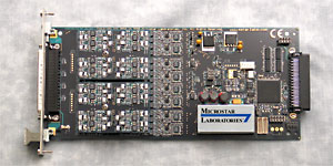
Figure 3 - MSXB 065 signal conditioning board
An MSXB065 differential signal conditioning and filtering board amplifies the low-level thermocouple signal, applying a gain of 25 and raising the signal range to approximately 0.1 volts. Despite best efforts to shield the signals from noise, some interfering noise will leak in and add to the inherently noisy readings from the thermocouple. A fourth order Butterworth filter tuned to a 500 Hz cutoff will remove all high frequency random noise from the measurements.
Applications with less stringent accuracy and speed requirements can route thermocouples directly to a termination board, with an onboard CJC circuit, and breadboarding space for termination networks.
The excitation and signal lines required for the thermocouple and supplementary cold junction sensors are provided through the 37-in panel connector of the MSXB 065. A balanced termination network on the board provides a ground reference voltage so that the thermocouple junction does not "float" to a high common mode voltage.
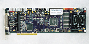
Figure 4 - DAP 5000a board
We will choose a DAP 5000a for the sampling and data processing. A DAP 5000a provides good support for numerical filtering operations, plus processing capacity for additional monitoring functions not covered here.
With less stringent measurement requirements, you would probably choose a DAP 840.
For supporting more channels and more complex calibration curves, you would probably choose a DAP 5200a.
The 100 millivolt signal level is still too small to digitize with good precision. Configure the input sampling of the Data Acquisition Processor to apply an additional gain of 40. This will raise the signal range to about 4 volts, within the usual +/- 5 volt input range used by most Data Acquisition Processor configurations. In the input configuration, your input channel definition will look something like the following:
SET IP1 D1 40
Over the temperature range of 55 degrees to 85 degrees, the response levels of the thermocouple range from 2.251 to 3.385 millivolts, so the range of variations seen by the converters are 2.251 to 3.385 volts. This is 1.134 volts out of the full 10 volt span — 1858 converter counts out of the 16384 counts available with a 14-bit converter. That gives a temperature resolution of 30/1858 = 0.02 degrees. If we presume that the last two bits of the converter are compromised by converter chatter and nonlinearity, that still yields measurement accuracy better than 0.08 degrees C.
Processing and digital filtering
Sampling at 1500 samples per second guarantees that any signal passing through the 500 Hz lowpass filter is accurately represented, including lower-frequency noise. We can use the following command to smooth the signal and reduce the sampling rate to a more friendly 150 samples per second for processing.
FIRLOWPASS(IP1, 10, PREDUCED)
After filtering, all noise beyond 75% of the Nyquist frequency (75 samples per second x 0.75) are gone. In particular, all 60 Hz interference from power sources is gone.
The 150 samples per second can still exhibit residual random noise in the 10 to 50 Hz range. We can apply digital filtering to remove most of that, with care. The lower the cutoff frequency, the more time delay in producing results. The 10 Hz cutoff is selected to keep this filtering delay relatively small. We can apply a 4th order inverse Chebyshev filter with 46 dB stopband rejection to remove the higher frequencies sharply while preserving the low-frequency temperature variations accurately. 10 Hz is 0.1333 of the Nyquist frequency of 75 Hz, so we specify the following digital filter.
CHEBYINV(PREDUCED, 4, 0.1333, 0.005, PFILT)
Calibration and conversions
The data stream PFILT above will have clean
measurements of thermocouple junction potential, but these
results must be converted into the desired temperature
measurements. We know that for a precision type-T thermocouple,
the response is almost linear in the limited operating range. If
we measure the thermocouple's output potential at the limits
of the operating range (55 degrees and 85 degrees C, call these
measured values POT55 and POT85), the following DAPL
expression can convert the measured junction potential
to the corresponding temperature anywhere in the range.
  LINTEMP = \
    ((POT85-PFILT)*55.0 + (PFILT-POT55)*85.0)) \
    / (POT85-POT55)
DAPL expressions look like simple arithmetic — but they actually define complete processing tasks that apply conversion operations to your entire data stream. Learn more.
The measurements used for the calibration include any effects from offsets and gain deviations in the amplifiers. So in additional to accounting for the thermocouple response, the calibration above also covers the measurement hardware. The usual approach of applying standard curves does not take measurement errors and sensor variations into account.
Unfortunately, the simple linear mapping as described above isn't completely satisfactory. From the standard type-T characteristic curve, we can learn that there is a maximum deviation of about -0.20 degrees from a linear curve in this range. We can easily correct for this effect, using an additional DAPL expression.
   TADJUSTED = LINTEMP + ( -0.20 * 4.0 *  \
     (PFILT-POT55)/(POT85-POT55) *        \
     (POT85-PFILT)/(POT85-POT55) )
You can verify that the second-order correction is zero at the ends of the ranges, and equal to the maximum -0.20 at the center of the range. The residual error in the corrected temperature reading is just a few hundredths of a degree. Thus, conversion errors are almost insignificant. Total system error depends almost exclusively on the quality of the signal and calibration.
The final temperature measurements are available 150 times per second, with a delay of a few milliseconds after receiving each temperature update. Total response delay depends almost exclusively on the temperature probe time constant.
Parts list (parts for thermocouple termination and cold junction measurement not included)
DAP
Analog Cable
Half IE with backplane
MSXB065 signal conditioning board