Using MSXB 067 Bridge Interface Boards
In Multi-Channel Vibration Applications
Technical Note TN-256 Version 1.0
The Vibration Measurement Problem
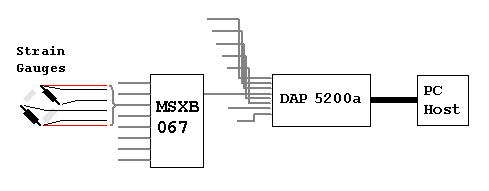
This technical note describes the problem of measuring vibrations in a metal frame structure. The structure will be subjected to disturbances through an actuator driven by a noise source. The vibration responses result in stresses that are measured by strain gauges. Low-level differential signals from the gauges are amplified on MSXB 067 Bridge Interface accessory cards, and delivered to the Data Acquisition Processor board as high-level signals. The Data Acquisition Processor then applies normalization and isolation filtering to the raw data, sending the finished and accurate strain data sets to the PC host for later offline analysis.
Measured Structure
For this example application, the structure to be measured is a frame for supporting a curved panel. The frame has six sections, so there are seven vertical ribs, running between two main horizontal beams, with various stiffening elements between. The stresses are measured at three points along each rib, near each end and near the center. There are also stress points monitored along each beam, at midpoints between vertical ribs. At each gauge position, the stress is measured in the vertical and horizontal orientations.
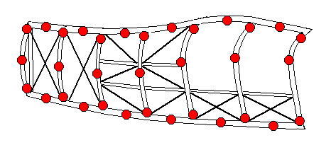
The final tally of strain monitoring gauges is:
(7x3 + 6x2) x 2 = 66 gauges
For each gauge, there is an amplified differential voltage, and this becomes a high-level differentially-driven signal that is transmitted to the Data Acquisition Processor. Various voltage drops and power interactions can occur on the excitation lines, but by measuring the excitation voltages simultaneously with the strain-induced voltages at each gauge, the disturbances can be compensated. The total so far is 132 differential channels.
To ensure that all vibration modes can be excited by the actuator, it is common practice to use a "white noise" signal, which over the long term produces a flat energy spectrum. However, the actuator has its own internal dynamics that will "color" the drive power spectrum seen by the test structure. It is advantageous to use a load cell to directly measure actual driving forces, adding two more differential channels for a MSXB 067 board bridge connection to capture. This increases the total hardware channel count to 134, still well within the capacity of 240 fully differential signals supportable in a single-DAP acquisition system.
Sampling Rates and Frequency Bands
The vibration frequencies considered important are the relatively low frequencies with the greatest potential for flexing the structure and producing damage. The analysis is restricted to 200 Hz or below. High-frequency secondary modes might have no direct importance, but they can produce highly correlated, repeatable effects that analog-to-digital converters will alias onto the low frequencies of interest, distorting the experiment results. To avoid problems of this sort, anti-alias filtering is required.
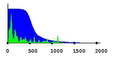
MSXB 067 boards with calibrated 500 Hz filters, MSXB067-01-500-E2Q01, are selected for this application. The filters have fourth-order Butterworth characteristics with the properties:
- < 0.1% maximum magnitude loss at the high limit of the desired 200 Hz band,
- attenuation to 1% or less of original levels at 1600 Hz or above,
- partial attenuation in the transition band from 200 Hz to 1600 Hz.
Rolloff characteristic of fourth order filters,
cutoff frequency 500 Hz
To avoid aliasing, the sampling rate must be high enough that frequencies within 200 Hz of the sampling frequency are attenuated such that they no longer matter. Selecting a sampling rate 2400 samples per second will do this, since the dangerous frequencies in the range 2200 to 2600 Hz are cut off by the analog filter. The sampling rate of 2400 samples per second is faster than the theoretical absolute minimum sampling rate of 400 samples/second necessary to accurately represent the desired 200 Hz band, but we must capture uncorrupted samples first. Later, digital processing can remove excess bulk from the data sets, leaving the desired band undistorted.
With 136 channels, each sampled at a 2400 sample per second rate, there is a channel-to-channel sampling interval of approximately 3 microseconds, which is well within the capability of a DAP 5200a.
Excitation Signal Generation
For this particular application example, we will assume that actuator drive signals are generated independently. Signal generation is mostly independent of the problem of capturing stress measurements. Still, there can be cases in which a Data Acquisition Processor offers advantages for drive signal generation, so we will cover this briefly.
To prepare a randomized drive configuration in DAPstudio, first configure an output updating procedure to drive the actuator command channel. Then add signal generation processing, something like the following.
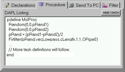
The filtering seen in this configuration can limit the excitation frequencies to the relevant bands, and compensate for actuator effects. The signal generation uses resources of the Data Acquisition Processor that would otherwise be idle, so in this sense, it is obtained "for free."
Preparing the Sensor gauges
For measuring low strain levels with best signal-to-noise ratio, the best configuration is the full bridge. The balancing circuit should be unstrained gauges of the same type, located physically and electrically close to the gauges that are strained. This is hard to do in practice, because every part of the frame will be stressed to some extent during testing.
Stable resistors mounted on the termination card are sometimes as good as you can do. We will assume here that each gauge set consists of an isolated matched pair. One gauge is configured into the upper half of the bridge, and one on the opposite side, producing roughly the equivalent of a full bridge.
Bridge Completion with Split gauges
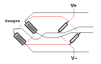
This configuration is covered in figure 11 of Technical Note TN-254 and you can find more information there. The resistors must be selected to approximately match the gauges in resistance and thermal characteristics, to produce approximate null output at no stress loading. For this application we will assume that the residual offsets are small, so that the signals remain within the linear range of the high-gain amplifiers. Frequency analysis might show a "blip" at zero frequency, but DC frequency is not of interest for the vibration analysis.
Packaging the Interface Boards
|
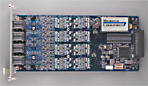
With 8 bridges supported per MSXB 067 board, the 66 gauges plus load cell will require 9 MSXB 067 boards. Each board will occupy two slots in a MSIE 002-06-P full size industrial enclosure, which means 18 slots of the available 21 slots are filled. An analog bus interface board is pre-installed in one of the three remaining slots, and the last two slots can remain covered. |
A cable MSCBL040-01-L18 joins the Data Acquisition Processor main analog interface connector to the analog backplane.
Part of the reason that MSXB 067 boards occupy double slots is to allow space for the 8 mini-DIN cable connectors. You can order MSCBL120-01K and MSCBL121-01K cable kits to be sure that you have compatible parts for wiring your cables.
Wiring Checklist
Wire the mini-DIN connectors to one end of the cables. Verify that the cables are correctly configured and shielded.
Bond the gauges to the correct locations on the test structure.
Connect the second end of the cables to the bonding pads on the gauges.
Mount the bridge completion resistors on your MSBCM001-01 completion module as illustrated in Figure 11 of Tech Note TN-254. Balancing resistor RA will connect from the plus supply XF+ to cable connection DF–. Balancing resistor RC will connect from the negative supply XF– to cable connection DF+.
Locate the J5 header on each MSXB 067 board, and configure the address jumpers according to the MSXB 067 manual, so that the boards are addressed as boards 0, 1, 2, etc. by the Data Acquisition Processor.
Populate your industrial enclosure with the MSXB 067 boards. Connect the analog cable to your Data Acquisition Processor.
Plug all of the mini-DIN connectors into the correct locations on the MSXB 067 termination boards on the panel of the industrial enclosure.
Connect the analog cable from the industrial enclosure analog backplane connector to the DAP analog interface connector on the card edge.
Configuring Data Sampling
The primary goal is to sample every gauge at approximately 2000 samples per second rate. Vibrations are not keyed to an accurate time base, so there is no special sampling rate ideally suited to detect them.
Capture. MSXB 067 interface boards require a "set up time" of at least 4 microseconds for accurate settling of the instrumentation amplifiers. However, we know that the channel-to-channel sampling interval is going to be about 3 microseconds. That's not enough for full measurement accuracy.
The default MSXB 067 configuration provides a solution for this. MSXB 067 boards do not capture bridge measurements in the Data Acquisition Processor address range D240 through D255. Instead, ALL MSXB 067 boards respond to a data read cycle in this range by beginning track mode operation — that is, the signals run through continuously, not latched as they would be during conversion. Then, when the Data Acquisition Processor begins a read cycle at any address outside of this range, ALL of the MSXB 067 boards latch and accurately hold their current levels, giving the effect of simultaneous sampling on all channels. The approximately 3 microseconds from channel to channel then relates only to the process of spooling the captured signals into the Data Acquisition Processor where there is plenty of time to do accurate conversions.
Sampling the high differential address twice (and ignoring the meaningless values reported) allows about 6 microseconds setup time. The two extra sampling intervals appear as two more logical channels in the sampling sequence, increasing the size of the logical channel list from 134 to 136, but the two extra values are ignored. DAPstudio provides configuration shortcuts to help you address the correct control channels.
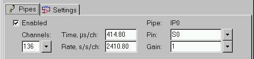
Timing. We now have complete information for configuring the input sampling using DAPstudio. Enter the count of 136 in the Channels box, and leave the gain level at the default level of 1. Enter the rate (samples per second on each channel) at 2400, and press Enter. Observe in the illustration below how DAPstudio adjusts the sampling rate to the nearest clock interval supported by the Data Acquisition Processor timing crystal. You will want to take note of the actual sampling rate, as this will affect the interpretation of the frequency spectrum later, but there is no difference to the effectiveness of the application. For applications where timing is much more important, adding extra "padding" channels to the channel list can align sampling rate more closely. Or you can provide your own external timing clock.
Gauge Signals. Next, configure the input
sampling channels for the actuator load cell and the strain
bridges. Right click on the channel display box on the left, and
choose "Select All" from the dialog. Left click on channels 0
and 1, to temporarily drop them from the display on the right.
In the display on the right, left click on the first channel in
the list, which will be logical data channel IP2. Above the
display, select "Differential" from the drop-down list for the
pin, and edit the pin number to make it 0. Leave the gain at 1.
Now, with pin IP2 still selected, right click on the display,
and select from the dialog "Selected Channels > Pin Increment
From First."
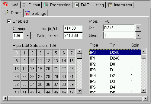
Latching Control.
Left click on the channel 0 and channel 1 boxes in the display
at the left. In the display on the right, logical data channels
IP0 and IP1 are now visible. Left click on IP0 to select this
channel. Above the display, select "D248 Track Mode" from the
drop-down list for the pin. Repeat these steps to configure pin
IP1. When you have finished this, your input sampling is
completely configured, and your input sampling configuration
screen should look something like the following.
Normalization and Excitation Disturbance Processing
For any given level of strain, the differential voltage output of a bridge circuit varies in proportion to the excitation voltage. The MSXB 067 power regulators will keep the excitation voltage as quiet and stable as possible, but there are typically small variations due to supply line drops, thermal resistance changes, loading changes induced by stress, inductive interference, etc. Thanks to the fact that we have accurately captured the excitation voltages at the same time as the bridge unbalance voltages, the variations cancel as measurements are normalized to the required "differential voltage per excitation volt" form. We will assume here that measurements of gauge excitation have no further use after normalization and are dropped, reducing the data volumes 50%.
Each MSXB 067 groups its hardware signals into two groups of 8, the differential strain voltage readings at channels 0 through 7 and the differential excitation readings at channels 8 through 15. The index sequence shifts upwards by 16 for the next board, and so on through the range. So, normalization involves pairs of channels with channel number differences of 8. We do not need to normalize the load cell measurement. We need some data pipes to contain the results of the normalization.
To avoid tedious data entry, we will use the features of DAPstudio to generate the normalization tasks. This will generate some extraneous lines, but highlighting and deleting these extra lines is relatively easy, compared to manually typing them.
Go to the configuration window in DAPstudio and select the
Processing tab. Select the Procedure sub-tab.
Place the cursor location inside of the Pdefine / End
processing group at the start of a blank line. Type the
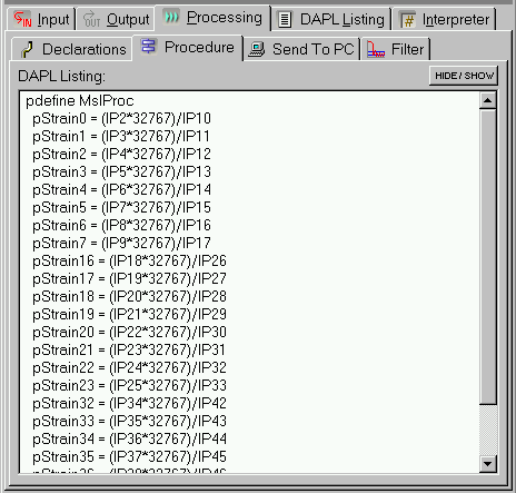
following DAPL expression task.
pStrain0 = (IP2*32767)/IP10
This instructs the DAPL system to set up a processing task
that generates a stream of normalized values. The constant
scaling term adjusts ratios in the range -1 to 1 so that they
are represented by the full integer range -32767 to +32767. The
logical data channels IP2 and IP10 are
the strain voltage and excitation voltage for the first gauge.
With the expression above highlighted, press the key
combination CTRL-C to copy it. Place the cursor on
a new blank line below the expression. Now begin pressing the
key combination CTRL-E. You can stop when you have
reached the last gauge differential signal at
pStrain129.
This process will generate the normalization task lines you need, but it will also generate meaningless operations involving the excitation from one gauge and the differential output of the next one. Clean up by deleting every second group of 8 task lines. This sounds like a lot of work, but you will find that it takes longer to read this explanation than to actually do it. When you get done with the cleanups, your processing screen will look something like the following:
Oversampling Reduction for Efficient Analysis
The 2400 samples per second rate used to capture the data set was deliberately set higher than the theoretical low bound, as discussed previously. In this case, the 2400 samples per second rate can be reduced by a factor of 3 to 800 samples per second, and still leave a good safety margin above the critical limit. This reduces the size of the data sets by 2/3, but preserves the frequencies in the range 0 to 200 Hz exactly, provided that no new aliasing is introduced by the decimation operation. Here, digital filtering serves the same purpose as the anti-aliasing filters for sampling the original continuous signals.
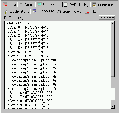
Return to the Processing sub-tab, and locate the curser on a new blank line. The order of the declarations does not matter for tasks, so you can insert the new task definitions just before the normalization tasks. Enter the following data reduction task definition:
Firlowpass(pStrain0,3,pDecim0)
Highlight this line and type the key sequence CTRL-C
to copy it. Once again, position the cursor on a blank line
below, and begin pressing the key sequence CTRL-E
until the last pipe pStrain129 is covered.
This construction has the same problems of generating extraneous lines, so once again, clean up by deleting every second cluster of 8 data reduction tasks.
The load cell measurement does not require normalization, but it gets the same benefits from data reductions. Add one more reduction task to the configuration. The filtered load cell signal is processed directly from sampled data.
Firlowpass(IP134,5,pDecim132)
After you have done all of the cleanups, your processing configuration will look something like the following. Lines have been rearranged so that the normalization and decimating filters are both visible, but such rearrangements are unnecessary in practice.
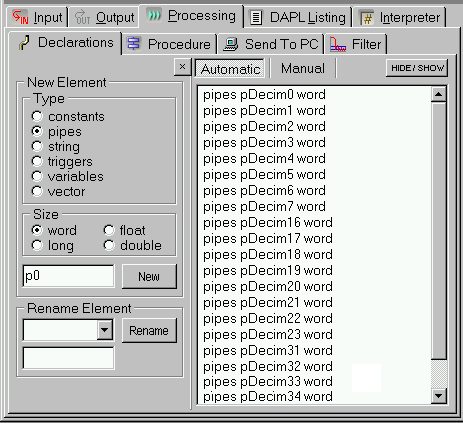
You might have noticed, the normalization tasks and the decimating filter tasks require new data streams for their results. DAPstudio is aware that these tasks will need these streams, and creates them for you. If you go to the Declarations subtab under the Processing tab, you can view the data pipes that DAPstudio has set up.
Data Logging
The data that you capture must cover an extended interval of time, so that there is a sufficient volume for an analysis to determine where strain magnitudes are greatest and whether the levels are acceptable. For this offline analysis, you must save measurement data to your host PC. You can achieve this easily using the data logging features of DAPstudio.
Under the Processing configuration tab, select the
Send To PC sub tab. At the upper right click the
clear all button. Then select the check boxes for each
pDecim pipe — the pipes containing the fully
processed data sets at a final 500 Hz sampling rate. Include the
load cell data. If you click on one of the names, and hold down
the left mouse key and drag across other names, you can highlight
several channels at once and activate them all by clicking
one of their check boxes.
Next, from the main window menu line, select Window |
New Disk Log. You will want to log all of the channels
that you configured to send to the PC host, so right click
anywhere on the display and choose Select All from the
pop-up dialog. Click the OK button to return
to the disk log window.
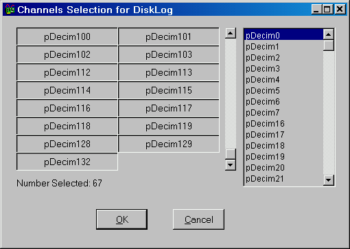
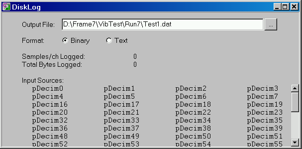
You will now see a display of all the channels to be logged to the disk file. Enter a path and file name in the text box at the top of the window. After that, logging to that file will begin automatically when the main menu Start! item is selected. The log file is closed automatically when the Stop main menu item is selected. Be sure to change the file name entry after each run to be sure you don't accidentally overwrite a previous data collection run (unless you want to do that).
Conclusion
A multi-channel, coordinated vibration data collection experiment can be a major undertaking, involving hundreds of sensor lines, hundreds of channels, and hundreds of processing tasks. Yet, as we have shown, setup for this experiment is relatively straightforward using the MSXB 067 bridge termination boards, packaged in an industrial enclosure, and configured using DAPstudio. If all you need is the data sets, you do not need to set up any additional software, as DAPstudio can log your data files efficiently.
The interface boards support the required arrays of anti- aliasing filters effortlessly. The differential instrumentation amplifiers for each channel make it possible to transfer clean high-level signals for fast digitizing conversions at full accuracy. The tedium of configuring acquisition software is mostly avoided, using some editing features of DAPstudio. You can validate your data, displaying the data channel by channel to verify correct operation, and then when everything is ready, run the full configuration and log the results. No additional pre-processing is required after data logging, as all of the low-level normalization, compensation, and raw data reduction processing you need can be done as data are collected, leaving data sets that are clean, accurate, and ready to analyze.
Now, if somebody could just figure out how to make strain gauge bridges that bond and wire themselves...
View other Technical Notes.