Accurate Trajectory Tracking with LMS Adaptive Filtering

Introduction

(View more Control information or download the preliminary implementation.)

Adaptive LMS filter tuning [1,2] is so deceptively simple that its effectiveness seems unlikely. Basically: if something works, do a little more of it. LMS adaption can be applied in many ways. We will show how to drive an LMS adaptive algorithm to obtain a feedforward filter that improves tracking of a continuously changing reference signal. We will show how adaptive tracking can be implemented in an existing control loop using just one additional processing command.

Example Application

The simplified hydraulic actuator drive system [3], described in another note on this site, is a severe test case. Its margin of stability is very poor, despite stabilization with a well-tuned multiple state feedback. This closed loop system is instructed to track a square wave, with sharp transitions that provide plenty of energy to excite poorly damped oscillatory modes.

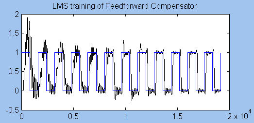
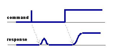
The following graph shows the response of the system as the feedforward compensation filter adjusts. As expected, the response is very ugly before training has tuned the compensation filter. After 20000 updates — that's four seconds — the oscillations are dramatically reduced. Notice the time delay.

Feedforward Control Strategy and Adaptive Learning

Patient: Doctor, it hurts when I raise my arm like this!

Doctor: Well then, don't raise your arm like that!

Feedforward control is roughly this same idea, but a little more practical. For good tracking, you want to avoid poor command signals that send your system into wild transients, while applying command signals that can move it effectively.

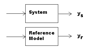
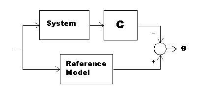
For tracking, the plant output should be neither too high nor too low, and a displacement of zero is a perfect match. One way to get this kind of "scoring" is to provide an ideal reference model and compare the actual system to this model.

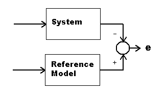
If we drive the actual plant and the ideal model with the same signal, perfect tracking will yield zero valued differences e.

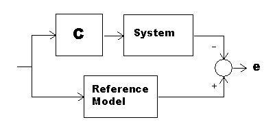
Clearly, if the plant and ideal model differ in any way, the tracking will not be perfect, and values of e will not be zero. Suppose that the plant is far from ideal. Interject filter C between the plant and the input signal. If this compensator filter C is an optimal feedforward controller, it achieves best possible tracking by forcing the combination of the filter and plant to match the desired ideal response characteristic.

Well, maybe a perfect match can't be obtained. But the smaller the differences, the better. Using the LMS algorithm, the sum of squares of the differences is driven as close to zero as possible.

Improving an Imperfect Filter

As an intermediate step to learning a good controller, consider the following variant of the previous configuration.

This seems rather pointless! The plant never sees the controller output. The motivation for this will be explained later. We know that if the plant is suitably linear, and we select a linear controller C, the reordered combination of plant and controller will yield the same combined output as before. We will use this configuration only to learn about the controller.

Now use a FIR filter — the same processing as in the DAPL system's FIRFILTER command — to implement the linear filter C. A FIR filter is defined by a vector of multiplier coefficients. These coefficients multiply the stream of present and past values, term by term, summing to yield the filter output.

Suppose that the current "score" value e is too high. That means, the controller output should be increased to improve tracking. By the LMS principle, we want to adjust the filter coefficients to produce a slightly more positive output. But there are lots of coefficients to adjust. How can we do this efficiently and consistently?

Here is where the LMS algorithm helps. It observes that given any arbitrary nonzero vector V, the vector dot product <V,V> will always yield a positive value. We can choose as vector V the history of filter input values from the filter shift register. The scaled vector e · <V,V> will then yield a result that is proportional to the current score and matching in sign. Now compare the vector dot product <V,V> to the FIR filter computation <V,C> . If we make C slightly more like e · V, this change is guaranteed to shift the filter output in the right direction. The cumulative effect of many small adjustments yields a greatly improved filter.

To summarize then, the μ-LMS algorithm selects a small step-scaling variable μ which it gets its name) to establish the adjustment size. After each new input the filter coefficients are incrementally improved using the update formula:

  C  <--- C  +  μ · e · V

There is one scalar multiply, one scalar times vector multiply, and one vector addition per update. We said deceptively simple, right?

The learning rate can be painfully slow, so variations of the LMS algorithm attempt to adjust the scaling variable and direction for faster convergence. Behind all of the variations, the principle remains the same.

Choosing an Ideal Reference Model

For a predetermined trajectory, there is a definite advantage to looking ahead, knowing where the system needs to go when determining how to move now. So allow a delay time. The filter must figure out how to best reach the target in the time available.

There is one practical problem associated with this. It is highly unlikely that the system will be able to track a single sample pulse perfectly. (Not that you would ever ask it to do that, right?) To make the filter a little less volatile, specify an impulse response that allows a little rounding at the corners. This is closely related to a windowing operation as applied in other DSP applications.

Combining Training With Control

Now at last it is time to clear up the mystery of the reversed controller and plant.

In previous discussions, the nature of the common input to the plant and to the ideal reference model was left unspecified. We will now specify it. This input is the output of the optimized controller C, driven by the desired trajectory signal. Unfortunately, the optimized controller filter is already occupied analyzing the outputs of the plant. What can we do about this?

Easy — apply digital magic. Make a copy of the trained coefficients. Use those same coefficients in another filter, thus obtaining the optimized drive signal. Apply that signal to the plant and to the ideal response model. Because the combination of the feedforward controller and plant has been adjusted by the LMS training, this should deliver the improved tracking performance.

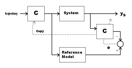
But wait, there is no point in physically copying the coefficient set. The second filter operation will not change the coefficient values. So all we really have to do is point both filter structures to the one coefficient set tuned by the LMS algorithm.

An Implementation: LMSMU Processing Command

The LMSMU processing command contains an implementation of the LMS algorithm as just described, with a few useful twists [4].

We know that in discrete control systems, frequencies more than about 20% of the Nyquist frequency are probably not helpful. So instead of keeping the exact past history in the training filter's shift register, LMSMU keeps a lowpass-filtered version of it. (Using filtered rather than raw history values is sometimes called the Filtered-X LMS algorithm.)
We want the LMSMU results to start harmless and improve from there. That is done by making the initial compensation filter a unit gain, passing the command signal through unchanged.
The response reference model is predetermined and fixed; it is the smoothed version of a unit gain response with delay.
The LMS algorithm works best when there is a strong correlation between values in the data stream over time. We know, however, that the impulse response of most systems decays over time, reducing the correlation. To concentrate on recent samples where correlation is likely to be the highest, positive "weighting factors" are applied to the LMS adjustments, favoring recent values over distant past ones.

The implementation needs three FIR filters, each operating on a different data stream, two of them sharing a common coefficient set trained by the LMS algorithm. The μ-LMS algorithm to train the shared coefficient set looks like the following.


  for  (i=0;  i<LENGTH; ++i)
    { LMS_coeffs[i] += 
      mu * err * LMS_weighting[i] * pShift[i]; }

The rest of the code fetches inputs, delivers outputs, and routes signals to the appropriate filters.

Processing Configurations

The LMSMU command packages all of the adaptive filter processing into one command. It uses two data input streams, the trajectory command signal and the plant output sequence. It has one output stream, the filtered command stream to send to the plant. The three FIR filters are all maintained internal to the command. To configure LMSMU, you must specify the desired length of the adaptive correction filter, the LMS correction step size μ, and the allowed delay time.

Suppose that the plant is stabilized using a PIDZ command [5] for feedback. The initial processing configuration might look like the following.


  PDEFINE  JUSTPID
    PIDZ( REFPIPE, IPIPE0, 12.8, \
      0.055, 0.0032, 0.75,  0.16666,\
      DRIVEPIPE, -32760, 32760)
    DACOUT( DRIVEPIPE, 0 )
  END

After adding an adaptive feedforward compensator:


  PDEFINE  ADAPTIVE
    LMSMU( REFPIPE, IPIPE0, CLENGTH, MU, DELAY, FEEDFW )
    PIDZ( FEEDFW, IPIPE0, 12.8, \
      0.055, 0.0032, 0.75, 0.16666, \
      DRIVEPIPE, -32760, 32760)
    DACOUT( DRIVEPIPE, 0 )
  END

The modified configuration treats the combination of the PIDZ stabilizer and plant as a single system. It learns the drive strategy to yield the best tracking performance for the closed loop combination.

If you would like to experiment with the LMSMU command, download it and try it with DAPstudio.

Conclusion

Perhaps the LMS adaptive tuning algorithm isn't exactly rocket science — but if it isn't, why do the rocket scientists use it so often? There are so many ways to use this simple technique that this note can barely scratch the surface. LMS training can be used to characterize system input/output response, predict future system actions, cancel background noise, improve feedback tuning, update recognition patterns... Sometimes the results are truly impressive.

There are some limitations. Though feedforward control can never degrade loop stability, it also cannot improve stability. Filter performance is uncertain with most nonlinear systems. [6] LMS learning is efficient and reliable but very slow, so it might not adapt fast enough to changing conditions.

The Developer's Toolkit for DAPL provides an excellent way to implement LMS adaptive techniques and make them accessible. As the LMSMU command illustrates, adding adaptive learning to an application can require only one additional configuration line. Feedforward compensation filtering is not a replacement for feedback control strategies like PID. Rather, it is a complementary technology. If you need better tracking, you just won't get it any easier than this. It might be worth a try.

Footnotes and References:

Adaptive Inverse Control, Bernard Widrow and Eugene Walach, Prentice Hall, Inc., 1996. Feedforward control is sometimes called inverse control because of the way it tends to cancel the natural dynamics of a controlled system. This book, by the originators of the LMS method, is highly readable and packed with good ideas from 25 years of application experience, but you won't find much specifically about tracking compensation there.
For a survey of adaptive filtering emphasizing the LMS method, "Introduction to Adaptive Filters", S. C. Douglas, chapter 18 in Digital Signal Processing Handbook, Vijay K. Madisetti and Douglas B. Williams editors, CRC Press, 1999.
DAPL Commands as State Observers - A Hydraulic Control Application, on this site. Hydraulics are wicked devices to control, and anything you can do to tame them is helpful.
Responses of physical systems can usually be described as a combination of "response modes" that are highly self-correlated but distinct from each other. These patterns might be identified by a principal component analysis, cosine transforms, singular value decomposition, self-organizing map, orthogonal polynomial decomposition... Training that emphasizes correlated patterns might converge better.
The PIDZ Command, on this site.
For nonlinear systems, replacing the linear FIR filter with a universal approximator such as a neural network might be effective.

Return to the Control page. Or download the experimental implementation.