Reducing Acquired Data

The most common reason for using a Data Acquisition Processor (DAP) board is its extended capacity. But if you use that capacity in the same way that you would use a basic data acquisition device, you will realize only a fraction of the potential benefits. This note is about using data acquisition effectively on a larger scale.

There are hardware and computing costs for capturing, moving, and processing data. The information content within the data might be considerably less than the bulk. Cost effective solutions will attempt to isolate the information content, so that resources are used more efficiently.

Cutting Large Problems To Size – Divide and Conquer

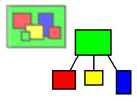
There are better ways to manage your needles than to pile them in haystacks. The more complex your data acquisition requirements, the more important it is to organize the application into manageable pieces, using a kind of layered organization.

The organizational decomposition principle: decide what to do at a higher level, perform the actions at a lower level. Higher levels provide lower level processes the resources needed to function. Lower levels provide higher levels with information needed to coordinate the processes.

Each removed piece of the problem is easier to deal with because it is small and isolated. The larger problem becomes simpler after the removal of the details that distract from the central mission. Applying the principle consistently to data acquisition applications results in host processing that gets the information it needs, rather than a lot of data with the information buried.

The Data Acquisition Processor board provides a processing resource that the executive functions can use. It is only a matter of utilizing it.

Preprocessing and Filtering

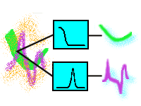
Consider an application that measures a process statistic over time, with measurements partially obscured by noise. To achieve the higher-level goal, first it is necessary to reduce noise content of the signal by filtering, and then to compute the statistics of the clean signal. The executive processing does not need to do all of this grinding, and should delegate the low-level activity to a "worker" task. Preprocessing takes measurements from the abstract digital form into the useful form that the application executive needs. This is something that you will probably have to do one way or another, and the sooner the better.

When signal noise is large enough that no individual measurement can be trusted to produce a representative reading, statistical approaches such as averaging must be used. Often, the sampling rates are boosted to capture enough data for meaningful control of measurement variances. The processing to get accurate information for the executive becomes much more intensive – all the more reason to use extra computing resources.

With the DAPL system, your higher-level application can request averaging for noise reduction, simply by requesting the following task in the DAPL processing configuration.

  AVERAGE( pSignal, cAvgBlock, pAverage )

You can then apply other pre-processing operations, such as offset and gain correction if you wish.

  SCALE( pAverage, cOffset, cSCale, pToHost )

Instead of streaming the bulk data into the host, clean, normalized values in meaningful measurement units can be delivered.

Data Selection

It is easy to run out of capacity in large-scale multi-channel measurement applications. Due to sheer volume, data can accumulate very fast. When every single measurement is important, in ways that can not always be anticipated, the best you can hope to do is record as much data as possible for later analysis. In other cases, though, you can be more selective.

There are two very common situations in which data can be taken selectively.

Periodically. Sometimes sampling rates must be set very high to capture the information of interest. But the process doesn't change very fast, so it is not necessary to repeat the analysis frequently. On Data Acquisition Processors, you can use the SKIP command to retain local bursts of data for analysis.
```
   // Select one block out of 50 for detailed analysis
   SKIP( pBULK, 0, 1000, 49000, pRETAINED )
```
Intermittently. Sometimes data of interest are associated with isolated events. You need lots of measurements when something happens, but nothing the rest of the time. On Data Acquisition Processors, you can use the LIMIT command (or any other event detection processing) with software triggering to determine when the data are meaningful. Then use the WAIT command to retain desired data for further processing.
```
   // Select bulk data when a threshold level is reached 
   LIMIT( pMonitor, inside,20000,25000, tEvent )
   WAIT ( pBulkData, tEvent, 0,1000, pRETAINED )
```

Visual Data Displays

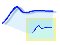
An important case of intelligent data selection involves graphical displays. Suppose that you have a data channel sampled at 10 microsecond intervals, capturing data in blocks of 1000 samples. You want to display data by block on a graphical plot. How much is useful?

Suppose that you have a moderate screen resolution with 1200 pixels width, with a graphical plot display that is half of the screen width at 600 pixels. One pixel can display one value along the vertical axis, while the horizontal axis represents the sequence. Thus the screen can display 600 resolvable values at one time.

To register with human vision, a display screen update needs to persist for about 1/20 of a second, otherwise there is only the slightest sensation of a flickering blur. Updating the screen 20 times per second would use 20 x 600 = 12000 values. That means that 88000 of the 100000 values produced each second cannot be displayed, even under ideal conditions.

Host computers are well suited for graphical display purposes, but giving 8 times more numbers than they can possibly hope to use is asking for problems. The graphical display software must make some difficult decisions about which data to display, which data to purge. And no matter how well it decides, it will not be able to make the best decisions all of the time.

Given that data will be discarded one way or the other, you can take some control, and perhaps avoid transferring a lot of data that cannot possibly be used well.

You can select data periodically, allowing sufficient time between updates for data to be displayed and observed.
You can select data when there is an indication that they contain something of interest.
You can also apply a mixed strategy, displaying interesting data when available, otherwise updating periodically.

DAPL software triggering supports a kind of mixed data selection strategy that is well suited for graphical displays. To use it, first determine how much data will be needed. Suppose for example that there are 100000 samples captured per second. Updating 4 times per second (once per 25000 input samples) can produce an acceptable display when there is nothing important happening. When there is anything interesting, the updates can occur as often as 10 times per second. To get these behaviors, the trigger is configured with an automatic cycle as follows:

  TRIGGER  mode=AUTO cycle=25000 holdoff=10000

Retain enough data for plotting at each event. Providing 600 to 1000 values per display update, rather than 25000, produces cleaner displays and leaves your application with more time for producing the results that matter.

Data On Demand

Another strategy for delivering data selectively is to wait until the host application is ready and asks for it. This is not the right way to observe a process continuously, but it is good for obtaining current and representative data quickly. Any data the host doesn't need are cleaned away automatically.

The idea is to use some of the storage capacity on the Data Acquisition Processor to preserve the most recent block of data. When the host sends a request message, that data block is sent immediately, using the MRBLOCK processing command. Because this data block is already in buffer memory, response to the request is almost instantaneous.

  MRBLOCK( pSourceData, pRequest, cBlockSize, pSELECTED )

Knowing that data will be provided immediately, some tricky timing-related code can be avoided in your application code.

Monitoring and Liveness

Sometimes the purpose of measuring is not specifically to record the measurements, but rather to verify that the data collection processing is proceeding normally. For this kind of application, there is really no point in tying up the host bus with data transfers that should never have anything to show. Data Acquisition Processors can perform this kind of testing for the host quietly, in the background, reporting results in a manner similar to other kinds of data reduction processing:

Periodic. Periodically verify that tests are running and results remain reasonable.
As needed. Inform the host when test results are outside of acceptable limits.
On demand. Allow the host to request the latest test results for inspection at any time.
Combined strategies.

Rate Normalization

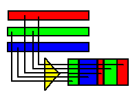
Generally, the signal needing the highest degree of time resolution will determine the sampling rate. Once this is established, it determines the rate at which samples are collected on all data channels. That doesn't mean that all of these data are useful. Data Acquisition Processors can use sampling configurations and processing to reduce the number of redundant samples when there is a mix of fast-changing and slow-changing signals.

In the sampling configuration, select a sampling rate that is faster than the minimum to obtain the required time resolution. For example, suppose a time resolution of 100 microseconds is needed. Use 50 microseconds for the sampling interval. Two such intervals equals the desired 0.1 millisecond interval for the high-resolution signal.

Next, for each of the slower channels, determine a timing interval that is a multiple of the sampling interval and sufficient for the channel. Suppose that the application has four additional channels that change slowly, so that sampling each one at 10 milliseconds intervals is sufficient. The slow channels can be sampled once per each set of 20 sampling intervals.

Now assign physical signals to the logical sampling sequence. For the example,

the high resolution signal is sampled every second interval,
the four low resolution signals are sampled every 20th interval, and
arbitrary signals are sampled at any remaining unassigned intervals.

The input sampling configuration looks like the following:

  idefine   multirate
    channels  20
    set ipipe0    s1     // SLOW CHANNEL
    set ipipe1    s0       // high rate sampling
    set ipipe2    s0       //   (ignore)
    set ipipe3    s0       // high rate sampling
    set ipipe4    s0       //   (ignore)
    set ipipe5    s0       // high rate sampling
    set ipipe6    s2     // SLOW CHANNEL
    set ipipe7    s0       // high rate sampling
    set ipipe8    s0       //   (ignore)
    set ipipe9    s0       // high rate sampling
    set ipipe10   s3     // SLOW CHANNEL
    set ipipe11   s0       // high rate sampling
    set ipipe12   s0       //   (ignore)
    set ipipe13   s0       // high rate sampling
    set ipipe14   s0       //   (ignore)
    set ipipe15   s0       // high rate sampling
    set ipipe16   s4     // SLOW CHANNEL
    set ipipe17   s0       // high rate sampling
    set ipipe18   s0       //   (ignore)
    set ipipe19   s0       // high rate sampling
    time  50
  end

The DAPL system allows you to extract the high resolution data from a combination of data channels.

The combined input channel pipe data stream
IPIPE(1,3,5,7,9,12,13,15,17,19)
will contain samples measured every 2 x 50 microseconds from the high-speed signal source.
The slow channels IPIPE0, IPIPE6, IPIPE10, and IPIPE16 will contain samples measured every 20 x 50 microseconds from individual channels.

Another strategy is to allow the Data Acquisition Processor to sample in a more uniform manner, selecting only the necessary data from data buffers.

 
  SKIP (IPipe0, 1,1,1, pHighRate)    
     // Retain one of two samples
  SKIP (IPipe1, 0,1,999, pLowRate1)    
     // Retain one sample of 1000
  SKIP (IPipe2, 0,1,4999, pLowRate2)    
     // Retain one sample of 5000

You can also use the two approaches in combination.

When you are using digital filtering for lowpass-and-decimate operations, you can achieve a similar effect without SKIP commands. The FIRFILTER command (and its cousin the FIRLOWPASS command) can reduce the number of filtered output values as part of its ordinary processing. In the following example, one value is retained for each 100 input samples collected.

  FIRFILTER ( IPipe(3,7,11,15), VFilt,65,1, 
     100, 0, pFiltered )

Logging Data

There are times when you really do need to retain and analyze all of the data. You have no choice but to spool as much data as possible across the main host interface to storage on disk drives. But it can be tricky to observe the progress of very high-speed transfers without interfering and impairing the transfer capacity.

The DAPL system has two ways it can help the host processing avoid extraneous processing in the critical data transfer loops.

Let the DAP extract the supervisory information and add it as a supplemental tag for each data block. In the following configuration, the tag consists of a sample count and an average value. No testing or searching is necessary. The host simply grabs these two values before sending each block of 10000 values for logging.
```
  NMERGE (1,pStartSample, 1,pAvgBlock, 10000,IPipe(0..49), 
     $Binout)   
```
You can completely eliminate extra coding from the high-speed data logging loop by configuring the DAPL system to send supervisory data on a separate channel. A supervisory thread on the host can read this data independently. On the DAPL processing side, the configuration might look something like this:
```
  COPY (IPipe(0..49), $Binout)
  MERGE (pStartSample, pAveBlock, Cp2Out)   
```

Conclusions

Simple data acquisition applications using simple acquisition devices in basic configurations don't need to be reduced. But for hard problems, when you need a DAP and all of its channel capacity and processing power, an everything-at-once approach leads to entangled applications where unrelated concerns interfere with each other: difficult to understand, difficult to test, difficult to optimize. Data reduction removes the redundancy from raw measurements, performing the bulk of the routine "number crunching" operations at the direction of the supervisory software. Supervisory application software receives the information it needs, when it need it, leaving more resources to concentrate on high-level tasks. This approach to organizing a data acquisition application is directly supported by the DAPL system, so it is always available. All your application has to do is ask for it.

Data Reduction: Isolating Information from Bulk Data

Introduction